Chapter 9: The rulebook and first workspace
Listen in Dr. Leith’s voice
Here is a strange thing about the work of the last eight chapters. You have a research question, a theoretical frame, a prospectus, a field-notes document, and a draft codebook. You have, in other words, designed an entire study around the Twitch dataset. And you have never actually seen it.
You have been told what it contains. Chapter 1 described a collection of nearly 1,700 channels recorded across five and a half days of November 2018, Bob Ross streaming under Art while most of the platform played games. Chapter 2 showed ten rows of it. You have taken the rest on trust. This chapter is where the trust ends and the looking begins. By the end of it you will have typed a few lines of R, and the dataset will have stopped being a description and become an object sitting in front of you, one you can inspect column by column.
This is also the chapter where the book changes character. For eight chapters there has been no code, on purpose. Planning a study before writing a line of it is the discipline that makes the code worth writing. But the planning is done. From here forward the work is done in R, and Chapter 9 is the gentle start: it opens a workspace, it loads the data, and it looks. It runs no analysis and computes no result. First contact is its own task, and it is worth doing slowly.
The workspace
Before the data, the workspace. Chapter 2 argued that reproducible research lives or dies on traceability: a study someone else can rerun is a study built from files in known places, not from commands typed once and forgotten. A project is how that happens. It is a single folder that holds everything one study needs, the data, the code, the codebook, the written report, so that the whole study travels together and nothing depends on a file that lives only on your laptop.
The v2v package scaffolds one for you. A single call does it:
v2v::new_portfolio("twitch-portfolio")Note the v2v:: in front of the function name. It is not decoration. It tells R, and tells you, that new_portfolio() comes from the v2v package specifically, the set of tools this book ships. Every v2v:: call in the chapters ahead carries that prefix for the same reason: so that the package never becomes a hidden assumption, and you always know which tools are the book’s and which are R’s own.
Running new_portfolio() creates a folder with a structure like this:
twitch-portfolio/
├── twitch-portfolio.Rproj
├── _quarto.yml
├── README.md
├── codebook.qmd
├── analysis.qmd
├── data/
└── .Rprofile
You did not have to decide where files go, what to name them, or how to wire them together. That is the point. Where to put things is a real source of friction for someone opening a data project for the first time, and an hour lost to it is an hour not spent on the study. The scaffold removes the decision.
One more call confirms the workspace is sound:
v2v::setup()setup() checks that R, the packages this book depends on, and the project’s environment are all present and the versions agree. You met it once already, in Chapter 2, as the final step of installing the stack. It returns here as a habit worth keeping: run it when you open a project, and you find out about a missing piece before it interrupts you mid-analysis.
The rulebook becomes a document
Look again at the scaffold. One of the files is codebook.qmd.
In Chapter 8 you drafted a codebook on paper: a unit of analysis, three operationalized variables, a set of decision rules. That draft was an argument about how the study would measure things. Now it becomes a document in the workspace, the project’s rulebook, the reference every later step answers to. Move the Chapter 8 draft into codebook.qmd, give it a version line and a date, and render it the way Chapter 2 had you render a one-page Quarto document. Rendering a codebook is not busywork. A codebook that renders cleanly is a codebook with no broken structure, and a rendered codebook is one a second coder can actually read.
Calling this “finalizing” the codebook is slightly optimistic, and it is worth being honest about that. Chapter 10 will pilot the codebook, two coders applying it to the same messages, and piloting routinely sends you back to edit a category or sharpen a rule. What Chapter 9 finalizes is not the content of the rulebook but its status: it stops being a sketch in your notes and becomes the official instrument of the project, versioned, rendered, and ready to be tested. A draft you can revise is exactly what you want walking into a pilot.
First contact with the data
Now the data. Two lines bring it in.
library(tidyverse)

chat <- v2v::twitch_chat()
streams <- v2v::twitch_streams()
The first line loads the tidyverse, the collection of R packages this book uses for everything from inspecting data to drawing figures (Wickham et al., 2019). The next two lines load the dataset itself. v2v::twitch_chat() returns the chat data; v2v::twitch_streams() returns the stream data. The arrow, <-, is R’s way of giving the result a name, so chat and streams now refer to the two tables for the rest of the session.
Notice that the data arrives through a function call, not as a file you opened or a spreadsheet you imported. This is deliberate. A new R user’s first encounter with data is often a pile of path errors, the file is somewhere the code cannot find, the format is not what was expected. twitch_chat() and twitch_streams() are written to remove that entire category of problem: they reach into the v2v package, find the data that ships inside it, and hand it back, with no path for you to get wrong. Called with no arguments, as above, each returns the full working sample. They also accept arguments for later, when you want only certain channels or games, but first contact is the no-argument version. Load everything, and look.
It is worth being clear about what “everything” means here. This is not the entire 2018 collection. The full dump runs to tens of millions of rows and well over a gigabyte, too much to ship inside a package or to open comfortably on a laptop. What v2v ships, and what you just loaded, is a working sample drawn from the fifty-channel corpus Chapter 1 described: a subset large enough to be real and small enough to be fast. Every example in the chapters ahead runs against this sample.
A word about what happens when this does not work. Sooner or later a line of R you type will return an error instead of a result: a misspelled function name, a package not loaded, a stray bracket. This is normal. It happens to everyone who writes code, and it is not a sign that you are unsuited to the work. The V2V Hub keeps a common-errors cheat sheet for exactly these moments, listing the errors a new R user meets most often and what each one is telling you. From this chapter forward, when a line breaks, that cheat sheet is the first place to look. An error is information, not a verdict.
Data provenance as a methodological disclosure. First contact is a moment of exploration (load, inspect, describe), but it rests on a prior step: documenting the provenance of the data before the first line of analysis code runs. When you publish a study, you are making a claim about specific data collected under specific conditions at a specific time. “I collected Twitch chat data” is not a methods section. “I collected 14 days of Twitch chat from the top 10 most-viewed streams in the Just Chatting category, using Twitch API v2, between 2024-01-15 and 2024-01-28, saving raw JSON responses to data/raw/ before any processing” is. The difference matters because replication requires exact knowledge of what was done. Munafo and colleagues describe what goes missing when a study is discoverable but its methods are not legible:
“Poor usability reflects difficulty in evaluating what was done, in reusing the methodology to assess reproducibility, and in incorporating the evidence into systematic reviews and meta-analyses.”
Munafo et al. (2017, p. 4)
For the v2v package dataset, write a four-sentence data provenance statement that would satisfy a journal methods section, and note what information you would need that the package documentation does not provide.
Looking at the data
The data is loaded. The first question is simply what it looks like, and the tidyverse function for that is glimpse(), which prints every column of a table, its type, and its first few values.
glimpse(chat)Rows: 35,267
Columns: 5
$ id <int> 89, 551, 1033, 2094, 2803, …
$ channel <chr> "sodapoppin", "xqcow", "forsen", "sodapoppin", "xqcow", …
$ sender <chr> "madzee", "prometheanow", "spectre155", "itsjer", "laserfru…
$ message <chr> "???????????????????????", "TriEasy Clap TriEasy Clap TriE…
$ date <dbl> 1542578127023, 1542578135562, 1542578143610, 1542578157677…Five columns, 35,267 rows, and each row is one chat message. id is a number that uniquely labels the message. channel is the channel the message was sent in. sender is the account that sent it. message is the text itself. date is when it was sent.
Two things in that output reward a closer look. The first is message. The values are real, and they are not tidy. The first message is twenty-three question marks. The second is the word “TriEasy Clap” repeated over and over, a viewer pasting the same phrase many times. These are not errors in the data. They are what Twitch chat actually contains, and your codebook will have to meet them as they are. The second is date. It is a column of enormous numbers, marked <dbl>, R’s label for a numeric value. Chapter 8 classified this column as interval-level and flagged the catch: the number is a count of milliseconds since 1970, not a date anyone can read. Converting it into a real timestamp is a headline lesson of Chapter 11. For now it is enough to notice that the column is there and that, as it stands, it is unreadable.
The stream table is the same kind of object with different columns.
glimpse(streams)Rows: 32,276
Columns: 6
$ id <int> 4, 10, 18, 61, 105, …
$ channel <chr> "sodapoppin", "xqcow", "forsen", "giantwaffle", "sodapoppin…
$ title <chr> "Hello truckers\n44835158804929_2115841973", "…", …
$ game <chr> "Marble It Up!", "Just Chatting", "Artifact", "Rocket Leag…
$ viewers <int> 27934, 19381, 15300, 4697, 28076, …
$ date <dbl> 1542578200214, 1542578200240, 1542578200273, 1542578200423…Six columns, 32,276 rows, and each row is one snapshot of one stream at one moment: its title, the game it was filed under, its viewers count, and the date of the snapshot. The first row should look familiar. It is Sodapoppin’s channel, playing Marble It Up!, with 27,934 viewers, the exact row Chapter 2 used to open its discussion of reproducible data. The fifth row is the same channel a few minutes later at 28,076 viewers, the climb Chapter 2 asked you to interpret. You are now looking at the source of that example directly.
The title column shows the same messiness as chat. The first title has a line break inside it and a long string of digits, which is not what a tidy title looks like but is what some streamers actually type. Real data is like this, and noticing it now, before any analysis, is the entire reason for first contact.
Beyond seeing the columns, you can count things. The tidyverse verb count() tallies how often each value of a column appears. Asking it about game shows what the streams are filed under:
streams %>% count(game, sort = TRUE)# A tibble: 60 × 2
game n
<chr> <int>
1 Art 5298
2 Fortnite 3682
3 Just Chatting 2474
4 Hearthstone 2157
5 Pokemon: Let's Go, Pikachu!/Eevee! 1967
6 League of Legends 1952
7 Heroes of the Storm 1473
8 Counter-Strike: Global Offensive 1346
9 Rocket League 1321
10 World of Warcraft 920
# ℹ 50 more rowsThe %>% is the tidyverse pipe: it takes the thing on its left and feeds it to the function on its right, so the line reads as an instruction in order, take streams, then count its games. The result is itself a small table, sixty rows, one per game, sorted with the most frequent at the top. Sixty categories is more variety than a study can examine one by one, and the count makes the shape of that variety visible: a handful of games account for most of the snapshots, and a long tail of fifty more accounts for the rest. That shape will matter in Chapter 12, when you have to decide how to draw a chart that does not drown in sixty lines.
count() is also a quick way to confirm the data is the corpus you expect. Chapter 1 described a working corpus of fifty channels. A related function, n_distinct(), counts how many different values a column holds, and asking it about channel checks that claim directly:
n_distinct(chat$channel)[1] 50Fifty distinct channels in the chat table, and n_distinct(streams$channel) returns the same fifty. The data you loaded is the corpus the book has been describing since Chapter 1, no more and no less.
There is one further way to look, worth knowing even though this chapter does not lean on it. Typing a table’s name on its own, just chat, prints its first rows in a compact form. Running View(chat) opens the table in a spreadsheet-style viewer you can scroll. Of the options, glimpse() is usually the most useful for seeing a table’s shape at a glance, but printing, View(), glimpse(), and count() are all doing the same basic thing: looking, without changing anything.
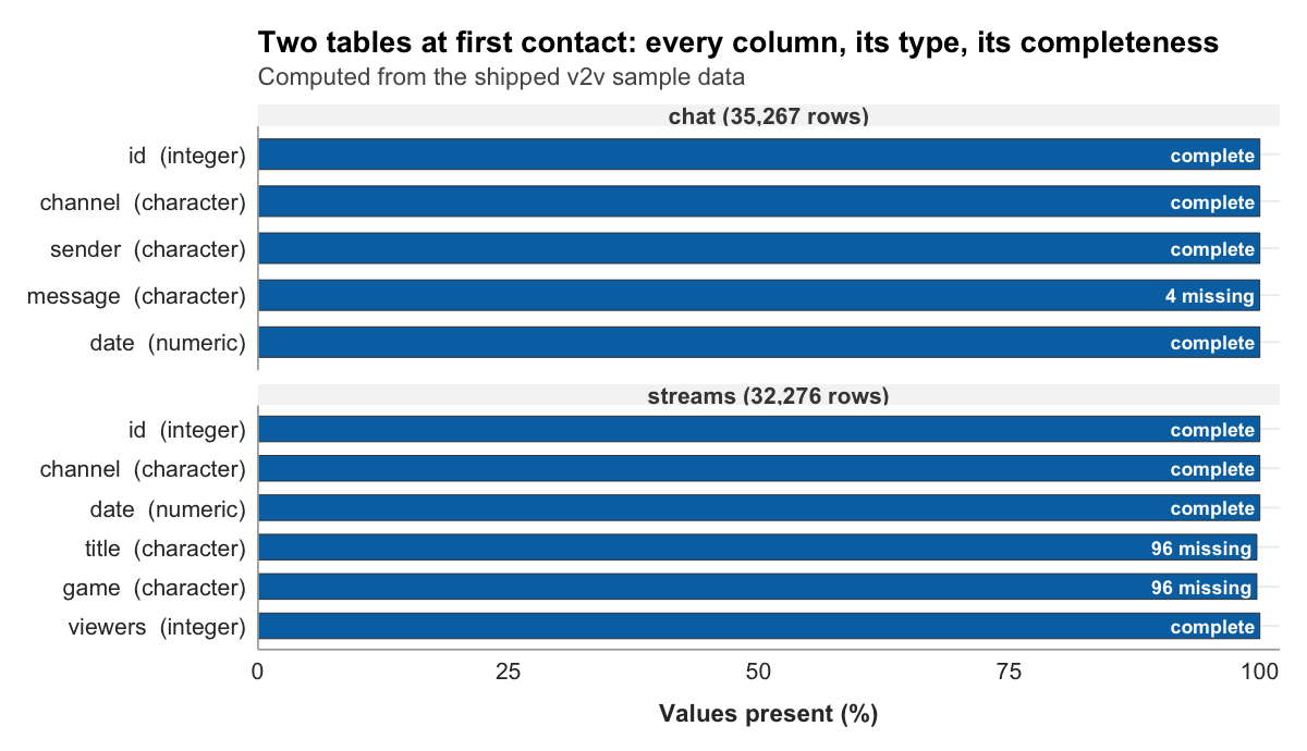
None of this changed the data. Looking is the whole of what this chapter has done with it. The chat table and the stream table are exactly as they were loaded. Inspection comes before transformation, and Chapter 9 stays entirely on the inspection side of that line.
Reading the data against the codebook
First contact has one job left, and it is the most important one. Open the codebook next to the glimpse() output and ask a blunt question: does this data actually support the study the codebook describes?
Walk the three variables. Message target is to be coded from each message, using the message text and, for at-mentions and replies, the sender information. The chat table has a message column and a sender column. Supported. Message length is the character count of the message string. There is a message column. Supported. Contains emote is read from the message text. There is a message column. Supported. The study the codebook designed is a study this data can carry. That is not a small thing to confirm, and it is far better to confirm it now than to discover a missing column halfway through coding.
First contact also surfaces what the codebook will have to work harder at. The messages in the glimpse() output are exactly the edge cases Chapter 7’s observation log anticipated and Chapter 8’s decision rules were written for. The message of twenty-three question marks is a message with no obvious target, the kind Rule 1 and the “unclassifiable” category exist to catch. The repeated “TriEasy Clap” is copypasta, which Rule 3 already addresses. Short tokens like the ones you can expect throughout the chat are emote-only messages, the subject of Rule 2. The codebook did not anticipate these in the abstract. It anticipated them because Chapter 7 had you watch for them, and here they are, in the first five rows.
One genuine wrinkle is worth carrying forward. Among the first messages is one addressed to a streamer: it begins “@xQcOW”. The channel column for that same row reads “xqcow”. The at-mention and the channel name are the same name in different casing, the display name as a viewer typed it against the lowercase login name the data stores. The message-target rule that keys on “an at-mention of the streamer’s channel name” will have to account for that difference. This is precisely the kind of refinement that belongs in the codebook now, while it is still the project’s living rulebook and before a single message has been coded. First contact has done its work: the study is buildable, and the codebook knows a little more than it did.
What the provenance record includes. For studies using the provided v2v package dataset, provenance is embedded in the package and stable. For studies using fresh API data, the record must include: (1) data source and API version; (2) date and time range of collection; (3) any filters, keywords, or channel selectors applied; (4) format in which raw data was saved; and (5) the git commit at which raw data was frozen (tagged as immutable). Item 5 connects directly to the audit trail: never re-run data collection to overwrite a file that a downstream script already depends on. If a journal reviewer asked you to share the raw data for a study using the v2v package dataset, consider what you would share and what you would withhold.
Looking ahead
You have a workspace, a rulebook installed in it, and the data loaded and inspected. Chapter 10 puts the rulebook to the test. It draws a sample of chat messages, the specific messages your study will actually code, and asks the question every content analysis has to answer before its results mean anything: when two coders apply the codebook independently, do they agree? Sampling and inter-coder reliability are the subject, and the codebook you finalized here is what goes on trial.
References
Wickham, H., Averick, M., Bryan, J., Chang, W., McGowan, L. D., François, R., Grolemund, G., Hayes, A., Henry, L., Hester, J., Kuhn, M., Pedersen, T. L., Miller, E., Bache, S. M., Müller, K., Ooms, J., Robinson, D., Seidel, D. P., Spinu, V., … Yutani, H. (2019). Welcome to the tidyverse. Journal of Open Source Software, 4(43), 1686. https://doi.org/10.21105/joss.01686
Graduate readings
Munafo, M. R., Nosek, B. A., Bishop, D. V. M., Button, K. S., Chambers, C. D., Percie du Sert, N., Simonsohn, U., Wagenmakers, E.-J., Ware, J. J., & Ioannidis, J. P. A. (2017). A manifesto for reproducible science. Nature Human Behaviour, 1, 0021. https://doi.org/10.1038/s41562-016-0021