Chapter 11: Wrangling the data
Listen in Dr. Leith’s voice
The chat table you loaded in Chapter 9 cannot answer your research question. Not yet. The study asks whether chat behaves differently on gaming and non-gaming channels, and it operationalizes that through message length. But look at the table. There is no column for message length. There is no column saying whether a message came from a gaming channel or a non-gaming one. The timestamps are unreadable runs of digits. And the information that would settle the gaming question is not even in the chat table; it sits in a separate stream table that the chat table has no link to.
This is the ordinary situation at this stage of a study, and closing the gap is the work of this chapter. Data wrangling is the process of turning the data you collected into the data you can analyze: reshaping it, cleaning it, deriving the variables your codebook named, and joining separate tables into one. It is unglamorous, it is rarely mentioned in the published paper, and it is most of the work. A wrangling chapter looks like a sequence of small technical steps. What it is actually doing is building the table that every later result depends on.
The verbs of data wrangling
The tidyverse handles wrangling through a small set of functions, each of which does one clear thing to a data frame. They are usually called the dplyr verbs, after the package they live in, and five of them carry most of the work.
filter() keeps rows that meet a condition and drops the rest. To look at only Bob Ross’s messages:
chat %>% filter(channel == "bobross")select() keeps or drops columns:
chat %>% select(channel, sender, message)mutate() adds a new column, or changes an existing one, computed from the columns already there. arrange() reorders the rows by a column’s values. And group_by() together with summarize() collapses many rows into one per group, which is how you compute a per-channel or per-game figure.
The reason these verbs combine so well is a shared design: each one takes a data frame and returns a data frame. That is what lets the pipe string them into a sequence, the output of one verb flowing in as the input of the next. A wrangling pipeline is just verbs chained this way, each step a small readable transformation, the whole chain carrying the data from raw to ready. The rest of this chapter is four such transformations.
The wrangling script as a methods section. A wrangling script is a documented transformation chain: a sequence of decisions, each recorded in version-controlled code, that connects raw data to analysis-ready data. Every mutate(), filter(), and group_by() is a methodological decision. You decided which cases to exclude and why. You decided how to handle missing values. You decided how to aggregate timestamp data into time windows. When a reviewer asks “how did you handle cases where the streamer’s username appeared in the chat?”, the answer is in the wrangling script, but only if the script is version-controlled and decision points are commented. For your own study, identify three wrangling decisions a reviewer might challenge, and for each add a comment stating the decision rule and its justification.
Making the timestamp readable
Start with the timestamps, because Chapter 9 already flagged them. The date column is a column of very large numbers, and Chapter 8 classified it as interval data with a catch: the number is not a date in any form a person can read.
What the number actually holds is a count of milliseconds elapsed since midnight on the first of January, 1970. That reference moment is the Unix epoch, the zero point nearly all computers use to keep time, and counting from it is how a timestamp becomes a single integer. The integer is precise and entirely unreadable. Turning it back into a date is a conversion, and mutate() is the verb for it:
chat <- chat %>%
  mutate(timestamp = as.POSIXct(date / 1000, origin = "1970-01-01", tz = "UTC"))
Two parts of that line carry the lesson. as.POSIXct() is the function that turns a number into a date-time value, given the origin to count from. And date / 1000 is the part it is easy to get wrong. as.POSIXct() expects a count of seconds, but the date column is a count of milliseconds, a thousand times finer. Hand it the raw number and it will place every message tens of thousands of years in the future. Dividing by 1,000 converts milliseconds to seconds first. It is a small arithmetic step and the single most common way this conversion fails.
Because it is the most common failure, the course package ships a wrapper that performs the division and the conversion together, so the mistake cannot happen by accident:
chat <- chat %>%
  mutate(timestamp = clean_dates(date))
That is the same operation, not a shortcut around it. clean_dates() exists to be read: run body(clean_dates) and you will find the line above. Use whichever you prefer in your own work, but learn the arithmetic first, because the day you meet a millisecond timestamp outside this course there will be no wrapper waiting for it.
The result is a real date-time. Setting date and the new timestamp side by side shows the transformation:
chat %>% select(date, timestamp) %>% head(3)# A tibble: 3 × 2
date timestamp
<dbl> <dttm>
1 1542578127023 2018-11-18 21:55:27
2 1542578135562 2018-11-18 21:55:35
3 1542578143610 2018-11-18 21:55:43The same instant, now legible: the evening of the 18th of November, 2018. The column type has changed too, from <dbl>, an ordinary number, to <dttm>, a date-time. That new type is what makes the column useful. From a real date-time you can pull the hour of day, the day of week, the calendar date, none of which can be read off the raw integer. Chapter 12 will use exactly that to chart how chat volume rises and falls across the hours of the day.
Measuring message length
The second transformation creates a variable the codebook named but the data does not yet contain. Message length, the character count of a message, is mutate() again, this time with str_length(), which counts the characters in a string:
chat <- chat %>%
  mutate(message_length = str_length(message))
chat %>% select(message, message_length) %>% head(3)# A tibble: 3 × 2
message message_length
<chr> <int>
1 "???????????????????????" 23
2 "TriEasy Clap TriEasy Clap TriEasy Cla…" 441
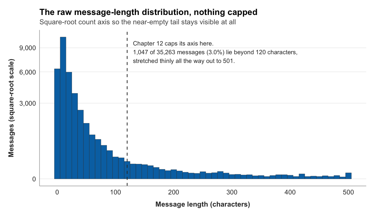
3 "cmonBruh" 8message_length is a ratio variable, in the Chapter 8 sense: a true zero, equal intervals, a count you can average and compare. The three values above also preview something. A single-word message of eight characters, a row of punctuation at twenty-three, and a block of copy-pasted text at 441 are all real Twitch chat, and the distance between them is large. That spread is the raw material of the study, and Chapter 12 will look hard at its shape.
Labeling gaming and non-gaming
The third transformation is the one the central research question turns on. Every message needs a label: did it come from a gaming channel or a non-gaming one? That label does not exist in the chat table, and building it takes more work than the last two, because the information lives in the other table.
Gaming or non-gaming is best understood as a property of the channel, fixed by what the channel mostly streams. Bob Ross’s channel streams painting; it is a non-gaming channel, and every message in it is a non-gaming message. So the label is built in three steps: find what each channel mostly streams, decide whether that counts as gaming, and attach the decision to every message from that channel.
The first step reaches into the stream table. Each channel appears there many times, once per snapshot, each snapshot carrying the game it was streaming. The channel’s dominant category is the modal category, the one that appears most often:
channel_type <- streams %>%
  filter(!is.na(game)) %>%
  count(channel, game) %>%
  group_by(channel) %>%
  slice_max(n, n = 1, with_ties = FALSE) %>%
  ungroup()
The pipeline reads in order. Drop snapshots with no recorded category. Count how many snapshots each channel logged in each category. Then, within each channel, keep only the single most frequent category. The result is one row per channel, naming what that channel streamed most.
The second step is a judgment, and it should be visible rather than buried. Twitch sorts streams into categories, and some of those categories are not games: painting under Art, unstructured talk under Just Chatting, and others. Listing them explicitly states the rule the study is using:
nongaming_categories <- c(
  "Art", "ASMR", "Beauty & Body Art", "Creative", "Food & Drink",
  "IRL", "Just Chatting", "Makers & Crafting", "Music",
  "Music & Performing Arts", "Science & Technology",
  "Sports & Fitness", "Talk Shows & Podcasts", "Travel & Outdoors"
)

channel_type <- channel_type %>%
  mutate(is_gaming = !(game %in% nongaming_categories)) %>%
  select(channel, is_gaming)
game %in% nongaming_categories asks whether a channel’s dominant category is on the non-gaming list; the ! negates it, so is_gaming is TRUE for every channel whose main category is a game and FALSE otherwise. channel_type is now a compact lookup table: one row per channel, one column saying gaming or not.
The third step is the join. A join brings columns from one table onto another by matching on a shared key, here the channel name. A left_join() keeps every row of the chat table and attaches the matching is_gaming value to it:
chat <- chat %>%
  left_join(channel_type, by = "channel")
A join is only as good as the match between its keys, and that is worth a word of warning. Twitch’s chat protocol writes channel names with a leading “#”, so the same channel can appear as #bobross in one source and bobross in another. Join two tables whose keys disagree like that and every row fails to match, silently. The v2v fixture has already normalized this, the “#” stripped before the data ever reached you, but raw Twitch data would need that cleaning step first. When a join returns nothing, mismatched keys are the first thing to check.
One result of the join deserves attention. Always inspect a column you just derived:
chat %>% count(is_gaming)# A tibble: 3 × 2
is_gaming n
<lgl> <int>
1 FALSE 3457
2 TRUE 31309
3 NA 501Two channels in the corpus streamed without ever having a category recorded: every one of their stream snapshots had a missing game. With no categories at all, there is no modal category, so those channels never made it into channel_type, and the left_join() left their messages with is_gaming set to NA. That is the correct outcome, not a bug. The data genuinely does not say whether those 501 messages came from gaming channels, and an honest NA records that the study cannot classify them. They will sit out the gaming comparison rather than being guessed into one side of it.
The analysis-ready table
Four transformations, run in sequence, have rebuilt the chat table:
chat <- v2v::twitch_chat() %>%
  mutate(
    timestamp = as.POSIXct(date / 1000, origin = "1970-01-01", tz = "UTC"),
    message_length = str_length(message)
  ) %>%
  left_join(channel_type, by = "channel")
A final glimpse() shows what the table has become:
Rows: 35,267
Columns: 8
$ id             <int> 89, 551, 1033, 2094, 2803, …
$ channel        <chr> "sodapoppin", "xqcow", "forsen", "sodapoppin", "xqcow…
$ sender         <chr> "madzee", "prometheanow", "spectre155", "itsjer", "la…
$ message        <chr> "???????????????????????", "TriEasy Clap TriEasy Cla…
$ date           <dbl> 1542578127023, 1542578135562, 1542578143610, 1542578…
$ timestamp      <dttm> 2018-11-18 21:55:27, 2018-11-18 21:55:35, 2018-11-18…
$ message_length <int> 23, 441, 8, 12, 206, …
$ is_gaming      <lgl> TRUE, FALSE, TRUE, TRUE, FALSE, …
This is what wrangling was for. The table is now tidy, in the precise sense the term carries in data science (Wickham, 2014): each row is one observation, a single chat message; each column is one variable; and everything the study needs sits in this one place. The unreadable integers have become timestamps. Message length and gaming status, named in the codebook and absent from the raw data, are now columns. The chat and stream tables, once disconnected, are joined.
None of this was analysis. Not a single result has been computed. But every result that follows, every figure in Chapter 12 and every test in Chapter 13, will be computed from this table, which is why the care spent building it is not optional. A wrangling mistake does not announce itself. It travels quietly into every chart and every statistic downstream. The reward for getting this chapter right is that nothing later has to be unwound.
Tidy data as the target state. Wickham’s tidy data principles (one observation per row, one variable per column, one value per cell) are not just a preference. They are the structural assumption that every tidyverse function makes about its inputs and produces about its outputs. Wickham (2014) defines the target in one sentence:
“Tidy data is a standard way of mapping the meaning of a dataset to its structure.”
Wickham (2014, p. 4)
Wrangling that produces tidy data is wrangling that can be audited: the structure itself is a transparency claim.
Never overwrite raw data. data/raw/ is read-only after the first commit. Your wrangling script reads from data/raw/ and writes to data/processed/. This separation means you can reproduce the processed dataset from scratch by re-running the wrangling script against the immutable raw data. Overwriting raw data severs this guarantee. To test the guarantee on your own study, re-run your wrangling script from a fresh R session against the raw data: if it does not produce the same processed dataset without manual intervention, find the undocumented dependency you missed.
Looking ahead
The data is tidy and the variables exist. The next move is to look at them. Chapter 12 turns the analysis-ready table into figures: how chat volume moves across the hours of the day, how viewership splits across game categories, and how the distribution of message length compares between gaming and non-gaming channels. It is the chapter where the study’s central question finally meets a picture of the answer.
References
Wickham, H. (2014). Tidy data. Journal of Statistical Software, 59(10), 1-23. https://doi.org/10.18637/jss.v059.i10